

2023-04-25
Inductance as an energy storage
«It was smooth on paper,
Yes, they forgot about the ravines…»
Stanislav Prokhorenko
Yes, they forgot about the ravines…»
Stanislav Prokhorenko
 This note is devoted to one interesting topic about inductance as an energy storage device.
There is an opinion that if you charge the inductance in portions, then the current in it will increase linearly, which means that as a result we will get an energy equal to the square of this current,
while portions of energy will need to be summed up.
It is known from mathematics that the square of the sum is greater than the sum of squares, and therefore, in this way, we will get an energy gain.
In this work, we will dispel this myth and show that it is impossible to get an energy increase for any values of intervals and portions.
Of course, this approach concerns only classical representations and does not take into account non-classical effects that may occur in LC circuits.
This note is devoted to one interesting topic about inductance as an energy storage device.
There is an opinion that if you charge the inductance in portions, then the current in it will increase linearly, which means that as a result we will get an energy equal to the square of this current,
while portions of energy will need to be summed up.
It is known from mathematics that the square of the sum is greater than the sum of squares, and therefore, in this way, we will get an energy gain.
In this work, we will dispel this myth and show that it is impossible to get an energy increase for any values of intervals and portions.
Of course, this approach concerns only classical representations and does not take into account non-classical effects that may occur in LC circuits.
What is it all about?
Let us assume that we introduce current into the inductor in portions, and after each such portion, the current grows linearly in it.
For simplicity, let's assume that the inductance \(L\) is 1 H, and each portion adds current \(I\) by 1 A.
Then the accumulated current for four (for example) portions will be equal to:
\[I_4 = I_1 + I_1 + I_1 + I_1 = 1 + 1 + 1 + 1 = 4\, (A) \tag{1}\]
The energy in the coil increases quadratically and at the end of 4 portions it becomes equal to:
\[W_L = {L\, I_4^2 \over 2} = {1 \cdot 4^2 \over 2} = 8\, (J) \tag{2}\]
On the other hand, each portion of the energy spent on the acceleration of the inductance is proportional to the square of the current separately, which in total gives the following result:
\[W_C = {L\, I_1^2 \over 2} + {L\, I_1^2 \over 2} + {L\, I_1^2 \over 2} + {L\, I_1^2 \over 2} = 2\, (J) \tag{3}\]
Attention: we spent 2 J of energy on charging the inductance, and received 8 J at the output.
The energy gain is 4 times, and if the number of servings is increased, then the gain will increase proportionally!
In mathematical language, it sounds like this: the square of the sum is greater than the sum of squares, which, in principle, is true.
Such reasoning can be found in some researchers of free energy.
In order for them not to go in this direction, and not to waste their precious time on this, we dedicated this work.
How it really is
To find the correct energy ratios of the energy expended and received, we will create an ideal installation,
where there will be no losses, and the pumping of energy in each portion will be implemented in the best possible way.
It is clear that then in a real installation, the efficiency will be even lower.
Figure 1a shows such pumping.
Here, the power supply U maintains the capacitor C in a voltage charged to the value \(U_C\), and it does this instantly, cost-free, and when the capacitance is disconnected from the inductance.
The UP block is responsible for this.
The capacitance is connected to the inductance using the SW block, which always connects it with the same polarity, because in the process of working with the inductance, it can be recharged.
This allows the current I to always flow in the same direction.
Thus, ideal conditions are created under which there are no losses and all energy flows into the inductance.

Fig.1. a) - scheme of idealized pumping of inductance L using capacitance C recharged from power supply U,
b) - diagram of the transient process for one portion of pumping (iteration)
|
Next, we consider one pumping portion (one iteration), the scheme of which is shown in Figure 1b.
For it, we have previously charged the capacitor to the voltage \(U_{C0}\), after which we closed the switch SW.
We can look at formulas for such a transition process in this work.
Since there are no losses in our scheme, we can use expressions (2.17) and (2.22), in which we assign: \(R = \alpha = 0\).
Let's rewrite these formulas taking into account our conditions:
\[ I = {U_{C0} \over Z} \sin(\omega_0 t) + I_0 \cos(\omega_0 t)
\\
U_C = U_{C0} \cos(\omega_0 t) - I_0 Z \sin(\omega_0 t)
\tag{4}\]
Recall that here \(I_0\) is the initial current in the circuit, \(U_{C0}\) is the initial voltage on the capacitor,
\(\omega_0 = {1 / \sqrt{L\, c}}\) is the circular resonant frequency, and \(Z = \sqrt{L / c}\), also called wave resistance.
According to Figure 1b: \(L\) is the inductance of the coil L, \(c\) is the capacitance of the capacitor C.
We constantly recharge the capacitance C and connect it to the inductor L, which already has the previously accumulated current.
Let us rewrite formulas (4) for such an iterative process:
\[ I_i = {U_{C0} \over Z} \sin(\omega_0 \tau) + I_{i-1} \cos(\omega_0 \tau)
\\
U_{Ci} = U_{C0} \cos(\omega_0 \tau) - I_{i-1} Z \sin(\omega_0 \tau)
\tag{5}\]
where: \(I_i, I_{i-1}\) is the current of the current and previous iteration, respectively, and \(I_0 = 0\) is the initial current before the start of the entire pumping process,
\(\tau\) -- time of one iteration, after which we will further calculate the current and voltage of each iteration step.
Let's temporarily simplify our formulas for better understanding, and introduce the following notation:
\[ \sin(\omega_0 \tau) = S, \quad \cos(\omega_0 \tau) = C \tag{6}\]
and we assign the value of unity to the initial voltage and wave resistance:
\[ U_{C0} = Z = 1 \tag{7}\]
Then the simplified formulas will look like this:
\[ I_i = S + I_{i-1} C
\\
U_{Ci} = C - I_{i-1}S
\tag{8}\]
Now let's see how the currents will be calculated at different iteration steps:
\[ I_1 = S
\\
I_2=S+I_1 C=S(1+C)
\\
I_3 = S + I_2 C = S (1 + C + C^2)
\\ ...
\tag{9}\]
One can see an obvious pattern for finding the current at the i-th iteration step:
\[ I_i = S \sum \limits_{n=1}^i C^{n-1} \tag{10}\]
To complete the picture, we also need to find the voltage across the capacitor at each iteration step.
From expression (8) we derive these values:
\[U_{Ci} = C - I_{i-1} S = C - S^2 \sum \limits_{n=1}^{i-1} C^{n-1} \tag {eleven}\]
An exception will be the case when i=1. We remember that \(I_0 = 0\), therefore: \(U_{C1} = C\).
This case occurs when we accumulate energy once (in one cycle), and although it will not be considered in reality, it was nevertheless necessary to pay attention to it.
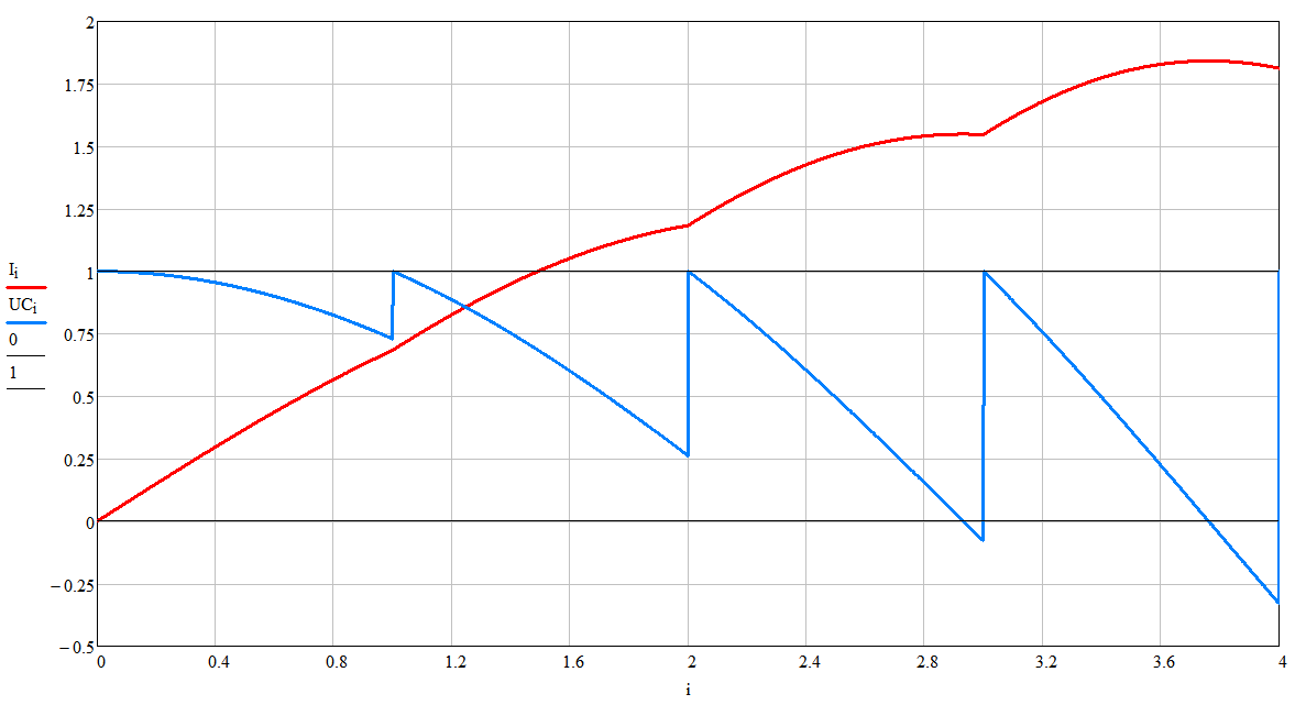
Fig.2. Graph of the growth of the current in the inductor I and the voltage across the capacitor UC at each iteration step (4 iterations)
|
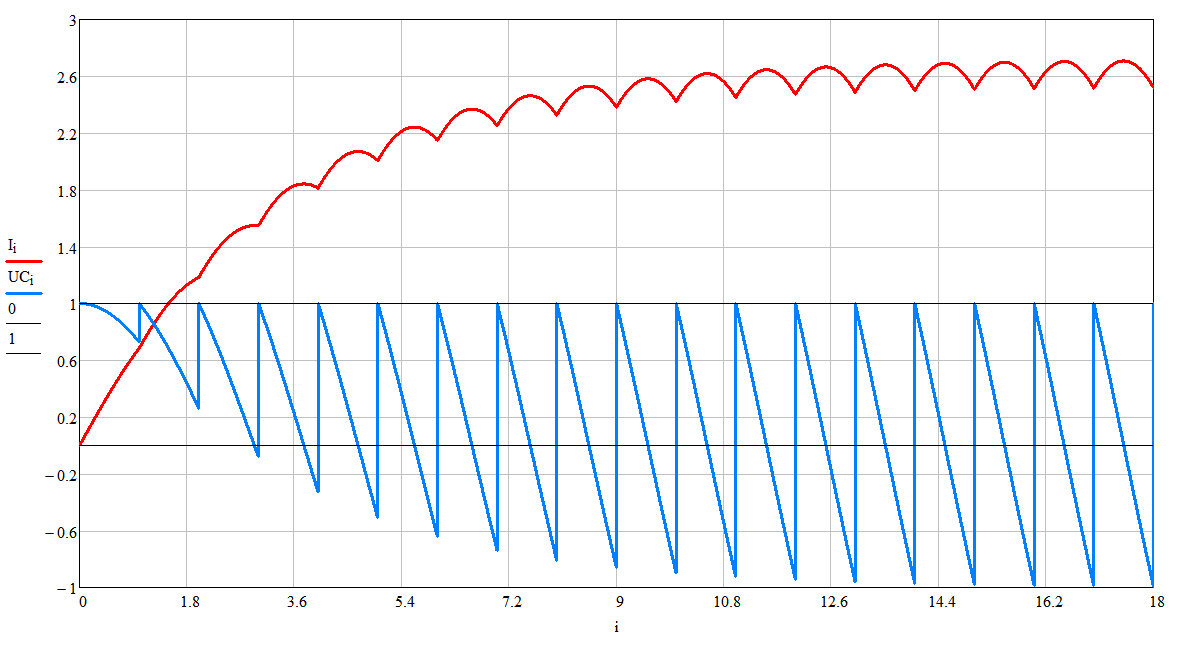
Fig.3. Graph of the growth of the current in the inductor I and the voltage across the capacitor UC at each iteration step (18 iterations)
|
Let's look at the graphs of the obtained functions (10) and (11), they are shown in Figures 2 and 3.
To build them, we took: \(\omega_0 = 2\pi, \tau= 0.12\).
On graph 2, one can find a relatively linear section of current growth at each iteration step, and the smaller \(\tau\) is, the more such points will be observed in the linear section.
But further, the current growth slows down, and the process gradually passes into a stationary mode (Fig. 3).
Energy balance and efficiency
Above, we calculated the current and voltage at any iteration step, and now, thanks to this,
we will be able to calculate the balance between the energy expended on the charge of the capacitance and the energy accumulated by the coil for any number of iterations.
Actually, because of the balance, this note appeared; he must show us the effectiveness of installations operating on this principle.
Recall how the potential energy of an inductance with current and the energy of a charged capacitor are calculated [1,2]:
\[ W_{L} = {L\, I^2 \over 2}
\\
W_{C} = {c\, U_{C}^2 \over 2}
\tag{12}\]
Now we just need to do the same as we did at the very beginning, in formulas (2) and (3).
At the i-th iteration step, the following energy will be accumulated in the inductor:
\[ W_{Li} = {L\, I_i^2 \over 2} \tag{13}\]
We recharge the capacitance at each iteration step again: from the voltage of the previous iteration to \(U_{C0}\).
Therefore, after each iteration, we spend the following energy on recharging the capacitor:
\[ W_{Cn} = {c\, U_{C0}^2 \over 2} - {c\, U_{Cn}^2 \over 2} \tag{14}\]
Then the total energy for recharging the capacitor in i iterations will be as follows:
\[ W_{Ci} = \sum \limits_{n=1}^i \left( {c\, U_{C0}^2 \over 2} - {c\, U_{Cn }^2 \over 2} \right) \tag{15}\]
From here we find the balance of energies, using the classical formula for efficiency:
\[ \eta_i = {W_{Li} \over W_{Ci}} \tag{16}\]
Since we agreed that while \(Z = \sqrt{L / c} = 1\), and \(U_{C0} = 1\), then the desired efficiency, for any number of iterations, is finally found So:
\[ \eta_i = {I_i^2 \over \sum \limits_{n=1}^i \left( 1 - U_{Cn}^2 \right)} \tag{17} \]
Here \(I_i\) is found by formula (10), and \(U_{Cn}\) is found by formula (11).
You can substitute the real values of capacitance, inductance and the initial charging voltage of the capacitor - the result will not change, and the formula will remain in the same form as it is presented in (17).
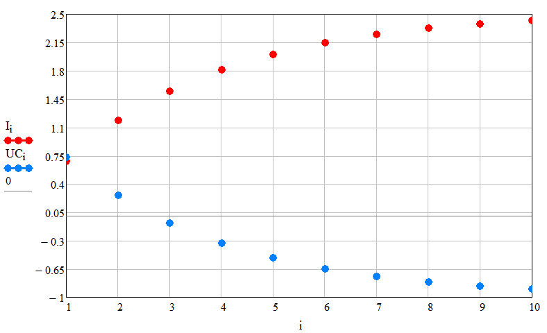
Fig.4. The values of the current in the inductor (red dots) and the voltage across the capacitor (blue dots) after the end of each iteration step, found by formulas (10) and (11)
|
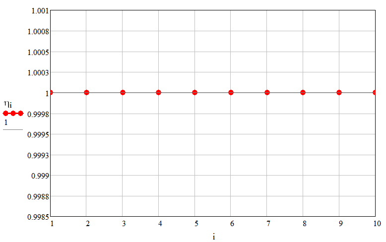
Fig.5. Efficiency values after the end of each iteration step, found by formula (17)
|
More clearly, these patterns are shown in Figures 4 and 5.
To build them, we took: \(\omega_0 = 2\pi, \tau= 0.12\), and the number of iterations: from 1 to 10.
But the efficiency value will be exactly the same for any number of iterations.
The exact proof of this is given in here.
Conclusions
It can be unequivocally said that for any values of inductance, capacitance, charging voltage and time of one iteration, the efficiency of this principle, at any iteration step, is equal to one
(see fig. 5 or this work).
Despite our expectations, nature disposed of its energy in its own way, presenting it in the original mathematics (formula 17).
In this note, we used ideal conditions, no loss. In reality, it will be necessary to take into account such losses and the efficiency of switching circuits.
Thus, the real efficiency of a device assembled on this principle will always be less than one.
Of course, this work does not take into account non-classical effects that can manifest themselves in such devices.
Calculating such phenomena requires a different mathematics, which is not presented here.
Используемые материалы
- Wikipedia. Inductance.
- Wikipedia. Capacitance.