

2023-08-10
A series with random signs and its sum
These series, according to the author, allow one to look into the future of quantum mechanics and explain some of the processes of this discipline from a purely mathematical point of view.
In addition, with their help, the line between a quantum and a non-quantum particle is generally erased, which can serve as a basis that unites two or more sciences.
But at the moment, such series have not been sufficiently studied due to the presence of random variables in them, which complicate their analysis.
The functions closest in meaning to the one we will consider further are the generating function of the sequence [1] and the random harmonic series [2].
But even they do not take into account all the nuances that arise when working with a random alternating series (SRS), to which this note will be devoted.
SRS is formed from the members of a series with a random sign in front of them:
\[A_n = \pm a_n x^n, \quad n \in 0,1,2,3,4,... \tag{1}\]
where: \(a_n\) is the nth coefficient of the series, \(x\) is some known value, which, as a rule, belongs to the following range of numbers: \(x \in 0.. 1\).
Sign values before \(a_n\) can be plus or minus with the same probability of ½.
But we will be further interested not in the series itself, but in its sum
\[f(x) = \sum \limits_{n=0}^{\infty} \pm a_n x^n \tag{2}\]
It would be possible to apply the generating function to such a sum [1], if the value of the sign in front of the coefficient of the series would have a certain regularity.
For SRS, the sum of a random harmonic series is also inapplicable [2].
But statistical mathematical methods of research are still available to us, and we will continue to use them, but first we will analyze a special case of the series stated above.
Investigation of the sum of SRS with the same members of the series
Before examining the generalized SRS, we turn to a simpler function of the form:
\[F_k = \sum \limits_{n=0}^{N} \pm 1, \quad k \in 1,2,3,4,\ldots, K \tag{6 }\]
where plus or minus before one can be chosen, in general, randomly, with probability ½.
The number of dimensions of the function \(F\) is equal to \(K\), and each such \(k\)-th dimension is stored in two arrays:
if the value \(F\) turned out to be positive, we enter it into the FP array, and if it is negative, then into the FM array.
A visual representation of two such arrays is shown in the following graphs:
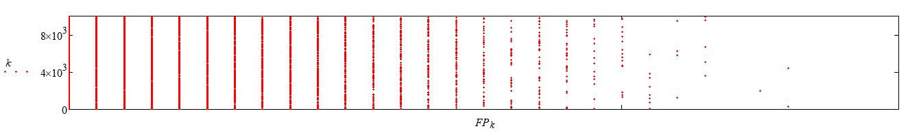
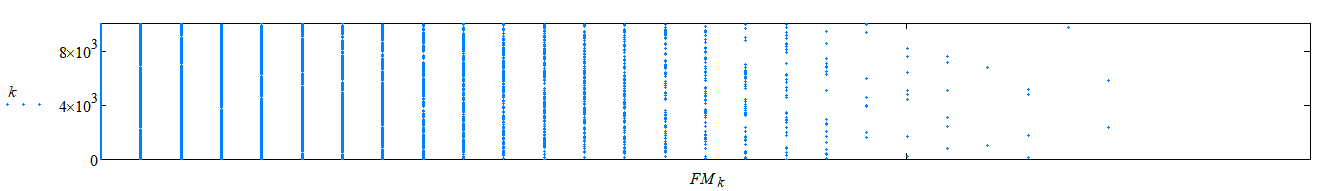
Fig.1. Positive (FP) and negative array data (FM) depending on measurement number k, at N=200 and K=10000
|
where each point is one dimension of the function \(F\).
But it is not very convenient to consider statistical data in this form, so science has come up with a special mechanism for this - a data histogram [3],
representing the frequencies with which the data falls within a certain interval (intrv).
An example from Figure 2: the function \(F\) equaled +12 about 400 times, and about the same number of times it equaled minus 12, for a total number of measurements of 10,000.
Such a graph is also called an energy spectrum:
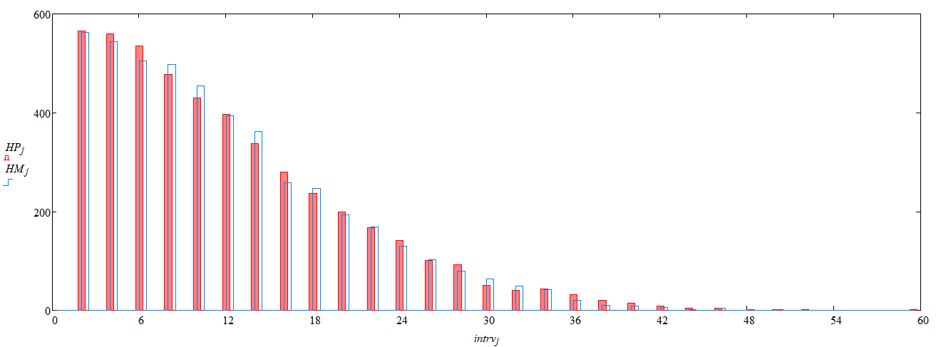
Fig.2. Spectrum of functions FP and FM, where HP are positive values, HM are negative values of functions, respectively
|
The spectrum of the F function corresponds to the normal Gaussian distribution [4], but with one nuance - the spectrum is discrete, not continuous.
And then the fun begins.
A random-sign-variable function gets a unit spectrum when we try to influence the arrangement of signs in a row.
For example, the function \(F\) will have a spectrum with one frequency if
\[F_k = \sum \limits_{n=0}^{N} (-1)^n \tag{7}\]
or
\[F_k = \sum \limits_{n=0}^{N} (-1)^{n+1} \tag{8}\]
Here we arrange the signs by introducing a certain regularity in their change.
Any such ordering brings the energy spectrum of the function to a unit value:
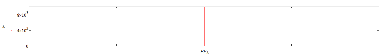
Fig.3. Distribution of the results of the F function according to the formula (7) or (8)
|
We got a completely different result (compare with Figure 1).But what has changed? Only the order in which we intervened!
Doesn't this look like a similar regularity when a particle passes through two slits [5]?
More general study of the sum of SRS
Consider the SRS in the form of a sum (2), but let's clarify the pattern for its elements:
\[F_k = \sum \limits_{n=0}^{N} \pm x^{2n} \tag{9}\]
Let's look at the test results of this function with their number: \(K=100000\)
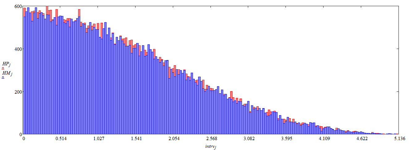


Fig.4. The spectrum of the f function, and the data of the results of the arrays FP and FM, according to the formula (9) with x =0.9
|
Let's reduce x to 0.75 and check the test results:


Fig.5. The spectrum of the F function, and the data of the results of the arrays FP and FM, according to the formula (9) with x =0.75
|
It can be seen that at x=0.75, some fluctuations appear in the spectrum (Fig. 5).
If you reduce x further, they become very obvious:
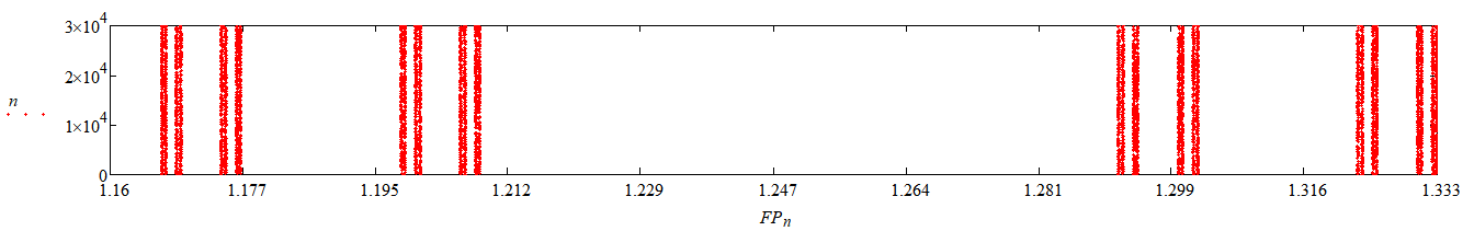
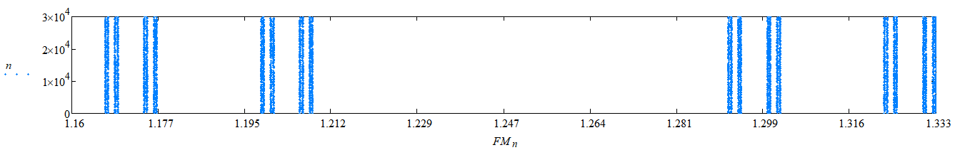
Fig.6. Result data of arrays FP and FM, according to formula (9) at x=0.5
|
If you reduce x further, then the discrete lines of the spectrum will become more and more clear, and the distance between adjacent lines will become less and less:
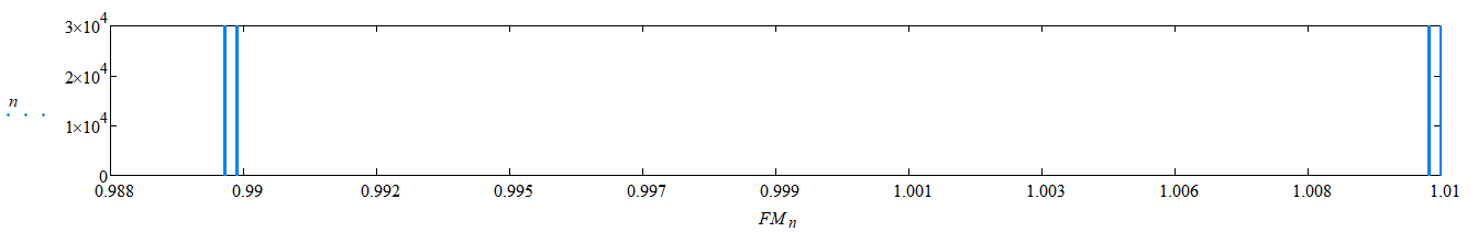
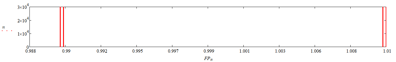
Figure 7. Result data of arrays FP and FM, according to formula (9) with x=0.1
|
As we can see, the differences between the data from the FP and FM arrays are practically the same.
Residual differences will fade as the number of trials increases.
Also, it is easy to see that the distance between the spectral groups is \(2 x^2\),
next in resolution is \(2 x^4\), then \(2 x^6\), and so on.
An example of a higher resolution spectrum is shown in Figure 8.
When x is close to unity, then all these lines practically merge into a single continuous spectrum (Fig. 4).
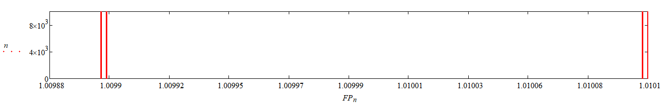
Fig.8. FP array result data, according to formula (9) and Figure 7, at x=0.1 (at higher resolution)
|
SRS Offset
The spectrum can be shifted to the right or to the left by setting the initial shift to formula (2).
In the following expression, we shift formula (9) by one
\[F_k = 1 + \sum \limits_{n=1}^{N} \pm x^{2n} \tag{10}\]
and get the corresponding spectrum plots:
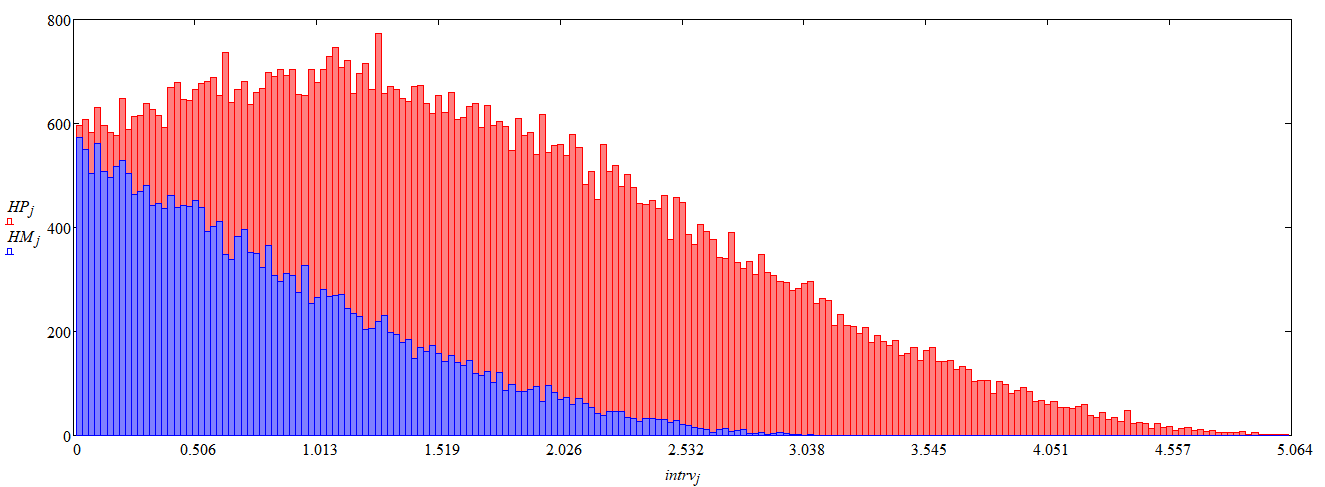
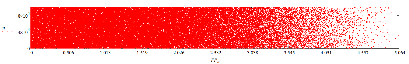
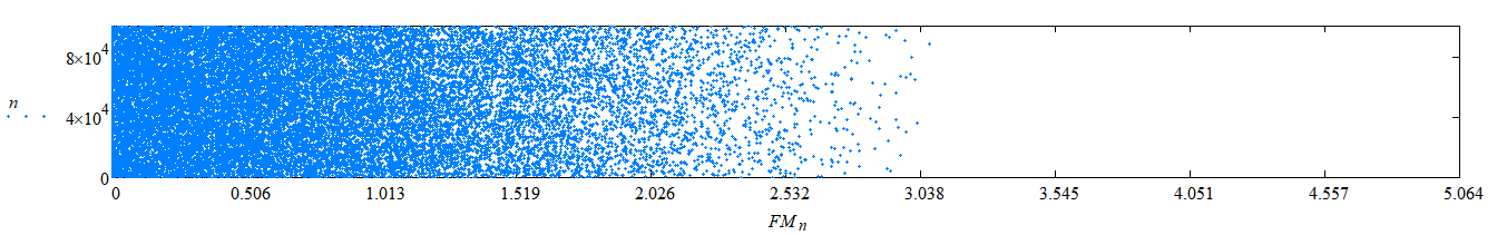
Fig.9. The spectrum of the F function, and the data of the results of the arrays FP and FM, according to the formula (10) with x =0.9
|
It goes without saying that the rule from (7-8) applies to all the spectra presented above:
if we interfere with the random order of plus and minus, then we get a unit spectrum as a result, as in Figure 3.
Sum of the SRS energy spectrum
The sum of the energy spectrum for the SRS can be represented as follows:
\[S = \sum \limits_{n=0}^{K} F_k \tag{11}\]
Sometimes it is required that such a sum be equal to some constant value.
For example, we want the following formula to
\[F_k = 1 + x^2 + \sum \limits_{n=2}^{N} \pm {x^{2n} \over n} \tag{12}\]
the sum of the spectrum was equal to one: \(S=1\).
Then, we can shift the probability of a minus or plus in front of the sum term of the series.
In this case, you need to increase the probability of a minus appearing over a plus by about 25 times:
\[F_k = 1 + x^2 + \sum \limits_{n=2}^{N} sign(rand(1.04) - 2) \cdot {x^{2n} \over n}, \quad S=1 \tag{13}\]
The energy spectrum graph of such a function will be as follows:
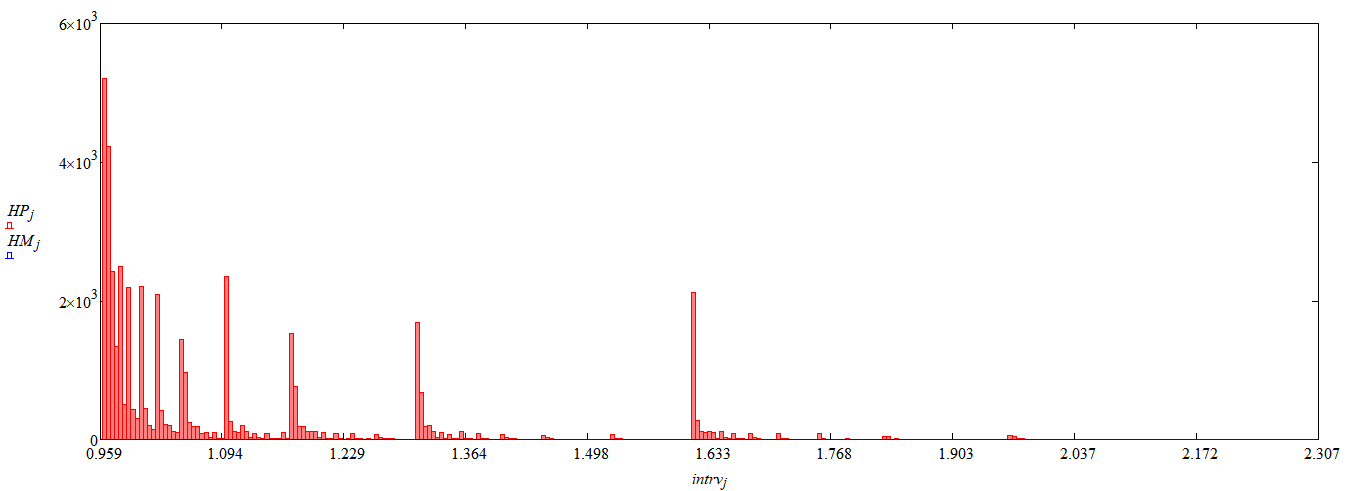
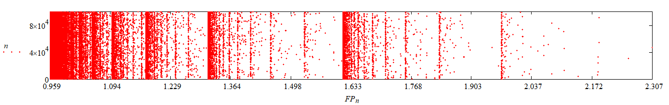
Fig.10. F function spectrum, and FP array result data, according to formula (13) at x=0.9. The sum of the spectrum according to (11) is equal to unity
|
Obviously, the array of negative measurement results FM is empty in this case and therefore is not shown in the figures.
Conclusions
In this note, previously little-studied random alternating series were presented and considered,
which can be applied, for example, to some applications of the single space theory.
It follows from them that the motion of a particle, in terms of its energetics, can be represented as the sum of such series.
If the energy of the particle should not change with any type of motion, you can use the sum of their spectra, which should be equal to some constant value.
If we don't want to destroy the SRS spectrum, then we can only partially influence the random choice of plus or minus in front of each member of the series.
But if the control of the appearance of these signs is complete, then we get a single degenerate spectrum, as in Figure 3.
This approach is reminiscent of the participation of an observer who intervenes in the experiment,
only here the observer influences the test through mathematics, changing the probability of the event.
When \(N\) tends to infinity, the SRS spectrum is also infinite in depth, and even if the spectrum is discrete (Fig. 7-8).
For spectra without probability shift, the author found the distances between the spectral lines at any resolution, which is equal to \(2 x^{2 g}\), where \(g \in 1,2,3,...\) - resolution depth.
Materials used
- Wikipedia. Generating function.
- Wikipedia. Harmonic series.
- Wikipedia. Histogram.
- Wikipedia. Normal distribution.
- Wikipedia. Double-slit experience.
- Gundina M. A., Yukhnovskaya O. V., Yukhnovskaya A. V. Implementation of the algorithm for generating random numbers in MathCad. [PDF]