

2026-03-14
Research of nanosecond high-voltage pulses
Nanosecond high-voltage pulses are of significant interest from both a practical and research perspective. Due to their short duration and high amplitude, such signals exhibit pronounced nonlinear interactions with conductive structures and the surrounding environment. They find application in pulsed electronics, electromagnetic radiation generation, and experiments involving fast transient processes in electrical circuits.
This paper examines an experimental study of a nanosecond high-voltage pulse generator and the characteristics of its interaction with a load and grounding circuit. Particular attention is paid to the observed effects associated with charge and energy redistribution in the system, which cannot always be explained within the framework of simplified equivalent models. The aim of this paper is to analyze these phenomena, quantify them, and discuss possible causes.
Preparing the Generator for Experiments
To conduct the experiment correctly, it is necessary to ensure galvanic isolation of the setup from the electrical network (Fig. 1). This is necessary to prevent the charges generated by the generator from leaking prematurely into the ground. This mode is achieved by powering the PHV voltage multiplier through the INV DC-AC inverter, which converts the 12V DC input voltage to 220V AC. The inverter itself can be powered either by a battery or by a network adapter with an output voltage of 12V.
 Fig. 1. Block diagram of the GNVIMP generator assembly for experiments |
The alternating voltage from the INV inverter output is fed to the PHV voltage multiplier, a detailed description of which is provided here. The high voltage from the multiplier output is fed to the GIHV converter, at the output of which nanosecond high-voltage pulses are generated. A similar circuit diagram of the device, but powered by a variable-frequency transistor transistor, was presented here. The electrical diagrams of these units, printed circuit boards, and configuration methods are also provided.
We have designated the combination of these units as the GNVIMP generator. Furthermore, this unit will be considered a single source of nanosecond high-voltage pulses and used in the experiments described below.
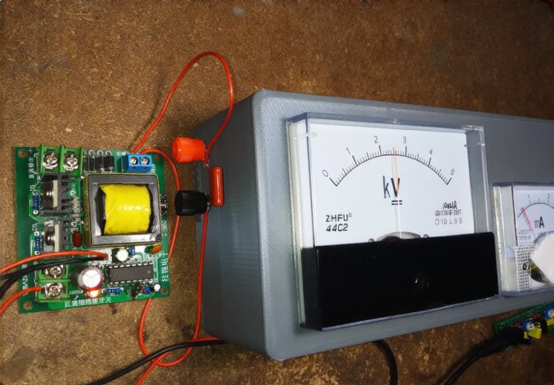 Fig.2. Photo of the INV inverter connected to the PHV multiplier. |  Fig. 3. Photo of the experiment with two antennas. |
A few words about the INV inverter. The author used a common DC-AC converter sold on Aliexpress under the name: DC-AC Converter Booster Module 12V to 110V 200V 220V 280V 150W. It allows the output voltage to be set to one of four values: 110, 200, 220, and 280 volts. 200 V proved to be optimal. To achieve this, a second jumper must be installed on the inverter board.
An additional 2 nF capacitor rated for 600 V (Cl in the diagram) must be connected to its output. It smooths the inverter's output rectangular pulses, which are sent at a frequency of 27 kHz, thereby significantly reducing interference. A photo of the inverter connected to the multiplier is shown in Fig. 2.
In this mode, the multiplier supplies approximately 2.5 kV (which is sufficient for avalanche mode in the GIHV converter) and a current of 0.5 mA to the circuit.
Conducting Experiments
The output of the GNVIMP generator must be left unloaded. Further experiments can be conducted with this (75 ohms), but the generator's free output will provide us with a more independent assessment of the output parameters.
 Fig.4. The probe lies next to the GNVIMP output |  Fig.5. Pulse on a grounded resistor Rr 100 Ohm |
We connect an antenna At to the output of the GNVIMP generator, which will be used in all subsequent experiments. It is a 15 cm long piece of copper wire, covered with a cambric (to prevent accidental contact). If you place the oscilloscope probe in the rows with this antenna, you can obtain an oscilloscope trace similar to the one in Photo 4.
Experiment #1. Two Antennas
The experimental setup is shown in Figure 6. This requires another antenna (Ar), exactly the same as the one on the generator. One end of the capacitor, Cr, goes through the generator's GND terminal, and a Vr voltmeter is connected to the capacitor, set to DC voltage measurement mode. The antennas are spaced at a distance of approximately 2-5 cm. A photo of the arrangement of the components for this experiment is shown in Fig. 3.
 Fig. 6. Experimental Schematic -- Two Antennas |  Fig. 7. Experimental Schematic -- Ground Current Oscillogram |
After turning on the generator, we can detect an anomaly in the form of stable negative values on the voltmeter. The order of magnitude is 100-200 mV, depending on the distance between the antennas and the length of the connecting wires. The voltmeter will show negative values even if the antennas are separated by several meters. Note: The voltmeter input must be high-impedance.
Experiment #2. Ground Current Oscillogram
The experiment diagram is shown in Figure 7. In this case, we connect a 100-ohm resistor Rr to the ground output of the GNVIMP generator, with the other end connected to ground. We connect the oscilloscope probe OSC1 in parallel with the resistor. The current oscillogram obtained in this experiment is shown in Figure 5. It shows that the voltage pulses across this resistor reach up to 200 V, and the current pulses up to 2 amps.
In the next experiment, we'll discover that a resistance of 100 ohms in the grounding circuit is not optimal for obtaining effective power.
Experiment #3. Power in the Grounding Circuit
To conduct this experiment, we'll also need to assemble a small circuit (Fig. 8), consisting of a diode bridge VDr, a resistor Rr, a smoothing capacitor Cr, and a voltmeter Vr. The diode bridge is connected across the generator-grounding circuit and rectifies the current flowing through it. However, the current actually flows through resistor Rr, the voltage across which we measure on the voltmeter connected in parallel to it. If this resistance is removed, the current to ground stops.
Thus, we can calculate both the average current and the average power going to ground. Here, another anomaly is revealed, since this power is approximately 4 times greater than what can pass through the radiating antenna At and, accordingly, go through ground. The average current, however, is many times greater than the calculated value.
Regarding the details, it should be noted that the author used high-speed diodes UF4007 for the diode bridge. A capacitor, ceramic, or any other SMD-capacitor rated for 100 V. Any resistor.
The optimal resistor value Rr is in the range of 40-60 kOhm. With a resistance of 51 kOhm, the voltmeter showed a voltage of 20 V, which translates to an average power of 7.8 mW. Further, we will show that an antenna of the specified dimensions can only handle no more than 1.3 mW.
 Fig.8. Experimental design - Power in the ground circuit |  Fig.9. Equivalent Circuit Circuit |
If we remove this resistor and switch the voltmeter to ammeter mode, we obtain values of approximately 3 mA, which is approximately 570 times greater than the average antenna current.
Calculations
To evaluate the obtained results, it is necessary to create an equivalent circuit (Fig. 9). The series circuit thus formed must include:
- Gi generator, producing pulses with an amplitude of 1000 V and a repetition rate of 1300 Hz;
- Ci capacitance, formed between the output of the HVIMP generator and ground. This is obtained by calculating the isolated capacitance of the antenna, which, given its dimensions, is approximately 3 pF;
- Ri resistance is 51 kOhm. It can be shown that in the equivalent circuit, with this capacitance and frequency, its value is not particularly important.
Let's find the average current through the charge stored in the capacitor Ci in one pulse. If the charge \(Q\) is full (and the circuit time constant is very small compared to the pulse period), then: \[\tag{1} Q = C_i\, U \] Considering a capacitance of 3 pF and an amplitude of 1000 V, we obtain \[Q = 3 \cdot 10^{-9}\, (C) \] Note: In this calculation, we assume the best-case conditions for the circuit. In reality, these values should be smaller.
We find the average current \(I_a\) as the product of the charge and the pulse repetition rate \(f\): \[\tag{2} I_a = Q\, f \] At a frequency of 1300 Hz, we obtain the average current: \[I_a = 2.6 \cdot 10^{-6}\, (A) \] However, if we take into account the charging and discharging of the capacitor, the current passing through the capacitor must be doubled: \[I_a = 5.2 \cdot 10^{-6}\, (A) \] But if the actual measured current is 3 mA, then the anomaly can be calculated by their ratio, that is, approximately 570 times.
Using a slightly different method, we can calculate the average power passing through the capacitor Ci. In this case, we first find the energy transferred by this capacitor to the load in each period: \[\tag{3} E_C = {C_i\, U^2 \over 2} \] To find the average power, we must multiply this energy by the pulse repetition rate: \[\tag{4} P_a = E_C\, f = f {C_i\, U^2 \over 2} \] With the parameters specified earlier, we obtain the average power passing through Ci, and therefore through the antenna: \[P_a = 1.95\, (mW) \] But if we calculate the power dissipated across resistor Rr (according to diagram 8), we get 7.8 mW. Which is approximately 4 times greater than the calculated value.
Note: We used the best possible parameters for the equivalent circuit. In reality, the obtained ratios may be even greater.
Conclusions
The results of the first experiment indicate a pronounced asymmetry in the processes associated with positive and negative charges. This is manifested in the appearance of a stable potential shift recorded by the measuring circuit. Similar effects have previously been observed, in particular, in a Tesla transformer under certain operating conditions. (see description). It can be noted that this effect intensifies with increasing pulse front steepness and amplitude.
The second and third experiments revealed that a pulsed current flows in the ground circuit, the magnitude of which significantly exceeds the current associated with the radiating antenna. At the same time, a power estimate shows that the energy dissipated in the ground circuit can be several times greater than the power transmitted through the antenna.
These results indicate that a simple model based solely on the capacitive coupling of the antenna to the surrounding space does not fully describe the processes taking place. It is likely that additional charge and energy transfer mechanisms are present in the system, requiring more detailed study.